Why You Can't Serve LLMs Like Regular Models (And How to Fix It)

If training an AI model is like sending a chef to culinary school for years, inference is putting that chef in a live Michelin-star kitchen on a Friday night at 8pm, taking real orders from paying customers who have expectations, dietary restrictions, and varying levels of patience — and delivering food that must feel magical every single time under extreme time pressure.

In the world of Generative AI, the single most important number is Tokens Per Second (TPS). A token is the atomic unit the model thinks in — roughly ¾ of a word on average in English. When you type a prompt and watch text appear, that streaming experience is the model emitting tokens one by one (or in small batches).

Good consumer experiences today sit in the 50–150 TPS range for small-to-medium models. High-end setups with heavy optimization can push 200–400+ TPS on dense models. Below ~30–40 TPS, the experience starts to feel sluggish. Below 15–20 TPS, users get frustrated and leave. Every extra token per second you can squeeze out of your GPUs is directly felt by every user.

Why LLM Inference Is Uniquely Difficult

Traditional machine learning inference (a ResNet classifying an image, a recommendation model scoring candidates) has very predictable characteristics:

• Fixed-size inputs (224×224 pixels, or a fixed feature vector)
• Fixed amount of computation per example
• Fixed-size outputs (a probability distribution over 1000 classes, or a single score)

Large Language Models break all three assumptions simultaneously:

• Variable-length inputs: A user can send 8 tokens or 128,000 tokens.
• Variable-length outputs: The model might stop after 12 tokens or keep going for 8,000.
• Autoregressive generation: Every new token depends on all previous tokens. You cannot parallelize the output the way you parallelize the input.

This combination creates five deep technical problems that simply do not exist in classical model serving. The rest of this essay exists to make you dangerous on all five.

The restaurant analogy: Traditional ML inference is a fast-food drive-thru. The menu is fixed, every car takes roughly the same amount of time, and the kitchen can plan perfectly. LLM inference is running the kitchen of a three-Michelin-star restaurant where one table orders a glass of water while the table next to them orders the full 18-course tasting menu with the wine pairing for every dish — and both tables expect their experience to feel equally special.

The Brutal Economics of Static Batching

In classical machine learning, the winning strategy for maximizing expensive GPU utilization is static batching: group several requests together and run them as one larger matrix multiplication. The fixed overhead of launching work on the GPU is amortized across many examples.

This strategy collapses with LLMs because of variable length computation.

Imagine you put four requests into a static batch:

• Request A: short prompt, generates 64 tokens
• Request B: medium prompt, generates 512 tokens
• Request C: long document, generates 2,048 tokens
• Request D: very long context, generates 8,192 tokens

Under static batching, the GPU finishes Request A after 64 steps but then sits mostly idle for the remaining ~8,000 steps while it waits for Request D. The three finished requests leave "holes" in the batch. Those holes represent extremely expensive silicon doing nothing.

At the scale of a real service (hundreds or thousands of requests per second), this waste compounds into millions of wasted GPU-seconds per day.

The Solution: Iteration-Level (Continuous) Batching

Modern LLM serving engines do something much more sophisticated.

They treat the batch as a fluid, living thing that is re-evaluated at every single decoding step.

The scheduler maintains a pool of active sequences. At each iteration it:

1. Decides which sequences still need work
2. Packs as many of them as will fit into the current batch (respecting memory and compute limits)
3. Runs one forward pass
4. Immediately evicts any sequences that just produced an end-of-sequence token
5. Instantly admits new sequences from the waiting queue into the newly freed slots

This is only possible because of a beautiful property of transformer decoders: once you have computed the KV cache for the first n tokens of a sequence, computing token n+1 only requires the new token embedding plus the existing KV cache. The engine can pause a sequence, swap it out of the active batch, and resume it later with almost zero wasted work.

This technique is usually called continuous batching or iteration-level scheduling.

Why This Matters in Production

Teams that moved from naive static batching (or even naive "one request per GPU") to proper continuous batching have reported 2–4× improvements in effective throughput on the same hardware, with no loss in latency for the average request. In some high-variance workloads the gains have been even larger.

This is not a small optimization. This is the difference between needing 200 H100s and needing 60 H100s to serve the same traffic.

Continuous batching solves the problem of idle time. But packing the kitchen so tightly creates a new, more subtle bottleneck: the work of preparing the ingredients (processing the full prompt in the prefill stage) has radically different resource characteristics than the work of plating one element at a time (the decode stage). This brings us to the second fundamental difference — and one of the most important architectural decisions in modern LLM serving.

The transition sentence from the previous section was deliberate. Once you embrace continuous batching, you quickly discover that not all work inside the batch is the same. Some work is extremely parallel and hungry for raw compute. Other work is painfully sequential and starved for memory bandwidth. Treating them identically is one of the most common (and expensive) mistakes in LLM serving.

The Kitchen Split: Prep Cooks vs Line Cooks

Continue the restaurant metaphor. In a real kitchen there are two very different kinds of work happening simultaneously:

• Prep work (mise en place): Reading the full order ticket, gathering and chopping ingredients, making stocks and sauces. This can be done in parallel by multiple people. Once the ingredients are ready, the actual cooking becomes much faster.
• Plating and finishing: The line cook actually cooking and assembling one dish at a time, plate by plate. This work is inherently sequential for a single order — you cannot plate the dessert before the main course is ready — and it is limited by how fast you can move things from the pass to the table.

LLM inference has an almost perfect analogue.

Prefill Stage: The Heavy Parallel Prep

When a request arrives, the model must first process the entire input prompt. This is called the prefill (or prompt processing) stage.

In the prefill stage the model runs a full forward pass over all input tokens at once. Attention is computed across the entire prompt in parallel. This phase has very high arithmetic intensity — lots of computation per byte of data moved. On modern GPUs it is almost always compute-bound.

Importantly, the cost is quadratic in the length of the prompt because of self-attention. A 4,096-token prompt requires roughly 16× more attention computation than a 1,024-token prompt (before you even count the feed-forward layers).

Decode Stage: One Token at a Time, Memory-Bound

Once the prefill is complete, the model switches to decode mode — generating output tokens one by one (or in small speculative batches in modern systems).

At each decode step the model only needs to compute attention for the single new token against all previous tokens (using the cached Keys and Values from earlier steps). The actual matrix multiplies for the new token are relatively small compared with the cost of moving the entire model weights and the growing KV cache from high-bandwidth memory (HBM) into the compute units.

This phase has very low arithmetic intensity. The GPU spends most of its time waiting for data to arrive from memory rather than doing useful math. Decode is almost always memory-bandwidth-bound.

Why Mixing Prefill and Decode Destroys Predictability

When you run both phases on the same set of GPUs (the default in many early serving setups), they fight each other constantly.

A long prefill job (someone pasted a 20-page document) can occupy a large portion of the GPU's compute resources for hundreds of milliseconds. During that time, every decode step for other users slows down dramatically because the memory bandwidth and compute are being stolen. Users experience unpredictable "jitter" — sometimes responses stream smoothly, other times they stall for a second or two.

In latency-sensitive applications (chat, agents, copilots), this tail latency is often worse than the average latency. Users remember the bad experiences.

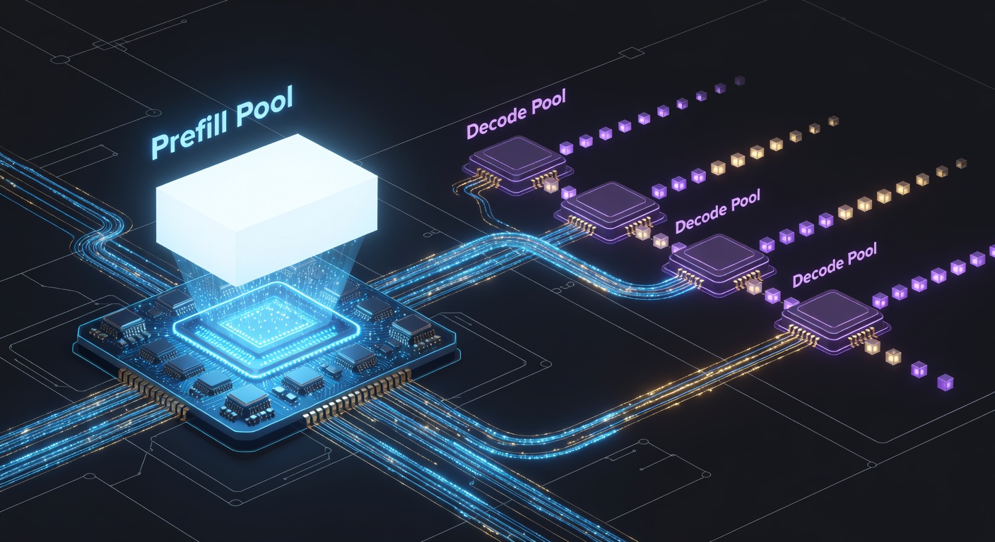
The Modern Solution: Prefill–Decode Disaggregation

The highest-performing large-scale systems now physically separate the two phases onto different pools of GPUs (or even different clusters).

Prefill pool: Optimized for high throughput and large batch sizes. These GPUs are usually packed with as much compute as possible (more SMs, higher clock speeds in some cases).

Decode pool: Optimized for low latency and memory bandwidth. These often use configurations that maximize HBM bandwidth per GPU and keep batch sizes smaller so each request gets predictable progress every few milliseconds.

When a prefill finishes, the resulting KV cache (or the minimal state needed) is transferred to a decode GPU, and the request continues generating there. The transfer cost exists, but for all but the shortest prompts it is dwarfed by the efficiency gains on both sides.

This pattern is now widely adopted. SGLang has excellent native support for it. Ray Serve + vLLM or TensorRT-LLM combinations are commonly used in production to orchestrate the handoff.

When to consider disaggregation: If your users are complaining about occasional long stalls during generation, or if you have a mix of very short and very long prompts, disaggregation is one of the highest-leverage architectural moves you can make.

Separating the two stages buys you much more predictable performance. But now every request that moves between pools carries with it a growing pile of state — the KV cache — that must be stored, managed, and eventually reclaimed. This state management problem is dramatically harder than anything classical model serving ever had to deal with. That brings us to the third (and arguably most important) difference.

Continuing the kitchen story: once continuous batching and disaggregation have made the line move efficiently, a new problem emerges. Customers are not ordering single dishes in isolation. They are having long, multi-course conversations with the kitchen.

Every time a regular customer returns and says "the usual, plus can I get the wine pairing this time?", the kitchen does not want to re-read the customer's entire previous order history from scratch just to remember what they liked last time. That history is extremely valuable state.

In LLMs, this state is the KV cache — and managing it efficiently is one of the hardest and most important problems in production serving.

What the KV Cache Actually Is

During the forward pass, the model computes Key and Value projections for every token at every layer (and every attention head). In the decode phase, instead of recomputing attention over the entire history from scratch for every new token, the model reuses these previously computed K and V vectors.

The size of this cache is linear in context length:

KV cache size (bytes) ≈ 2 × num_layers × num_kv_heads × head_dim × bytes_per_value × sequence_length

For a Llama-3 70B-class model (80 layers, 64 query heads but only 8 KV heads thanks to GQA, head_dim 128, FP16 = 2 bytes):

• One 8k context request consumes roughly 2.5 GB just for its KV cache.
• A batch of 64 concurrent 8k requests consumes ~160 GB before you even count model weights.
• At 128k context (increasingly common), a single request can easily require 40+ GB of KV cache.

This is frequently the largest memory consumer in high-concurrency serving, far larger than the model weights themselves for long-context workloads.

The Fragmentation Crisis

Early serving systems allocated the KV cache for each sequence as one giant contiguous block in GPU memory. This worked fine for short, uniform requests.

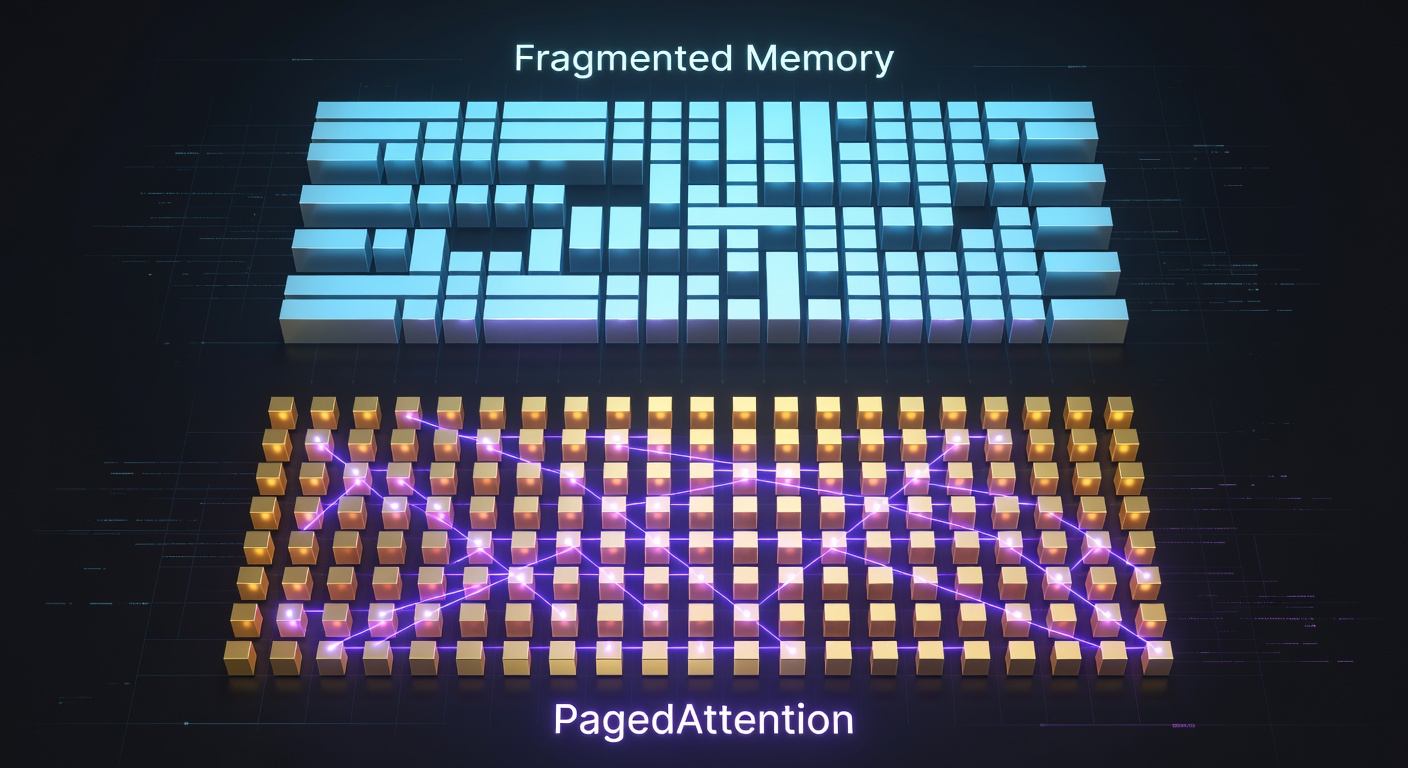
In the real world it collapses. Requests arrive and depart at different times with wildly different lengths. A conversation that started at 2k tokens might grow to 32k over 20 turns. Other requests finish and free their memory. You quickly end up with classic external fragmentation: plenty of free memory in aggregate, but no single contiguous slab large enough for a new long request.

This is the GPU equivalent of trying to seat a party of 12 when you only have scattered tables of 2 and 4 left.

The Breakthrough: PagedAttention (vLLM, 2023)

The vLLM team at UC Berkeley solved this by importing one of the most successful ideas in computer science: virtual memory and paging, invented in the 1960s for operating systems.

Instead of allocating one massive contiguous region per sequence, PagedAttention divides the KV cache into small, fixed-size blocks (typically 16 or 32 tokens worth of K/V vectors). These blocks can live anywhere in GPU memory. A lightweight block table (exactly analogous to a page table in an OS) keeps track of which logical blocks map to which physical memory locations.

Benefits:

• Elimination of external fragmentation — any free block can be used by any sequence.
• Efficient sharing of prefix blocks across multiple requests (the foundation for later prefix caching).
• Much higher memory utilization (often 80–95%+ instead of 30–50% in fragmented setups).

This single idea allowed vLLM to serve 2–4× more concurrent users on the same hardware compared with prior systems, and it became the foundation for virtually every serious open-source and commercial LLM inference engine that followed.

Beyond Paging: Real-World KV Cache Management

Paging solved fragmentation, but production systems still face hard questions:

• Prefix caching: When two requests share a long prefix (same system prompt + same uploaded document), can we share the KV blocks instead of recomputing them?
• Eviction policies: When memory is full, which sequences' caches should be discarded or swapped to CPU?
• Recompute vs cache trade-offs: For very long contexts in RAG, sometimes it is cheaper to drop old blocks and recompute them later than to keep everything resident.

Modern engines (SGLang's radix tree, vLLM's advanced prefix caching, TensorRT-LLM's features) combine paging with sophisticated prefix matching and eviction logic. This is no longer a simple cache — it is a full distributed memory management system for attention state.

Efficiently managing the KV cache is table stakes. But the cache is only valuable if you route new requests to the specific GPUs that already hold the relevant prefixes. Naively load-balancing without looking at what is cached destroys all the efficiency you just built. This is exactly why prefix-aware routing exists — and why it is the fourth fundamental difference.

By this point in the kitchen story, the implications should be clear. The most valuable thing in the restaurant is not the stoves or the plates — it is the institutional memory. The head waiter who knows that Table 7 always wants the sommelier's recommendation, that the couple at Table 12 had the 2018 Bordeaux last time and loved it, and that the solo diner at Table 3 is deathly allergic to pine nuts.

When a regular customer returns, you do not seat them with a random waiter who has never met them before. That would be terrible service and a massive waste of the head waiter's knowledge.

In LLM serving, the equivalent of that institutional memory is the KV cache. And most traditional load balancers are the equivalent of seating every returning customer with a random waiter.

The Expensive Mistake

Consider a typical RAG application:

• User uploads a 40-page legal contract or research paper (≈ 8,000–12,000 tokens).
• The system runs prefill, computes the KV cache for that document (this might take 2–8 seconds on a good GPU, depending on model size).
• The user then asks 15–20 follow-up questions over the next hour ("What does Clause 7.3 say about liability?", "Summarize the indemnity section", etc.).

Each of those follow-ups shares almost the entire prefix with the original document. If the load balancer sends the second question to a different replica than the first, that replica has to re-run the entire prefill from scratch. You just paid the full quadratic attention cost again for no reason.

In practice, this is one of the most common reasons "our RAG system is slow and expensive" — the system is recomputing the same expensive prefixes over and over because the router is prefix-blind.

How Prefix-Aware Routing Actually Works

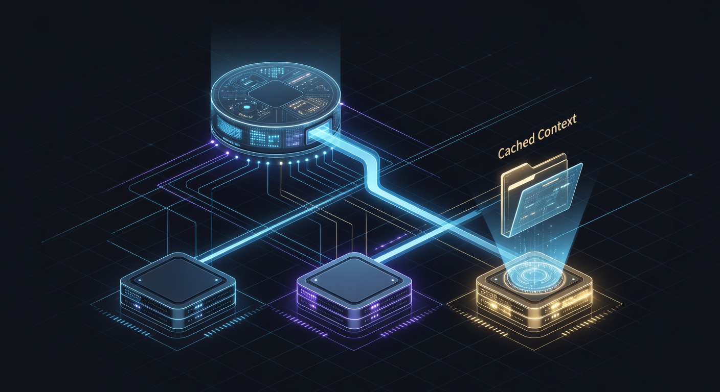
A prefix-aware router does not treat every incoming request as an independent unit. Instead, before deciding where to schedule a request, it inspects the prompt (or a compact representation of it) and asks: "Have we already computed the KV cache for any prefix of this prompt? If so, where is that cache currently resident?"

There are several levels of sophistication:

• Simple hash-based: Hash the first N tokens (or the system prompt + document ID) and route to any replica that has previously seen that hash.
• Radix tree / Trie-based (used in SGLang): Maintain a tree of all active prefixes across the cluster. This allows extremely fast longest-prefix matching and also enables efficient sharing of common prefixes between different users (e.g., the same system prompt used by thousands of users).
• Distributed prefix cache: The router (or a dedicated prefix cache service) keeps metadata about which nodes hold which prefix blocks. It can then either route the request to one of those nodes or, in advanced setups, migrate the relevant KV blocks to a less-loaded node.

The key insight is that the routing decision must happen *before* the request is assigned to a GPU. Once the request is already running on the wrong node, it is usually too late to fix without wasting the work that was just done.

Why This Is Harder Than It Sounds

Implementing good prefix-aware routing at scale introduces real engineering challenges:

• Prefixes are not always exact matches (a user might paste almost the same document with tiny formatting differences).
• The prefix cache itself consumes memory and needs its own eviction policy.
• In a distributed system, the router needs a consistent, low-latency view of where every active prefix block lives.
• There is a tension between maximizing cache hits (route to wherever the prefix lives) and load balancing (don't overload the one node that happens to have a popular prefix).

This is why you see specialized systems (SGLang's radix tree, custom routers in Ray Serve, various internal systems at large labs) rather than "just use Nginx or a generic load balancer."

Production Impact

In workloads with high prefix overlap (most real RAG applications, multi-turn agents, coding copilots with repository context, etc.), good prefix-aware routing can easily deliver 3–10× better effective throughput and dramatically lower latency for follow-up turns. It is one of the highest-leverage optimizations once you are past the basics of continuous batching and PagedAttention.

We now have efficient ways to keep the kitchen moving (continuous batching), separate the heavy prep from the delicate plating (disaggregation), and remember everything the customer has ever said without wasting memory (PagedAttention + prefix caching). But what happens when the recipe book itself is so large and specialized that no single chef can possibly know the whole thing? This is the world of Mixture-of-Experts models — and it forces us into the fifth and final fundamental difference.

We have now reached the final and most structurally different challenge.

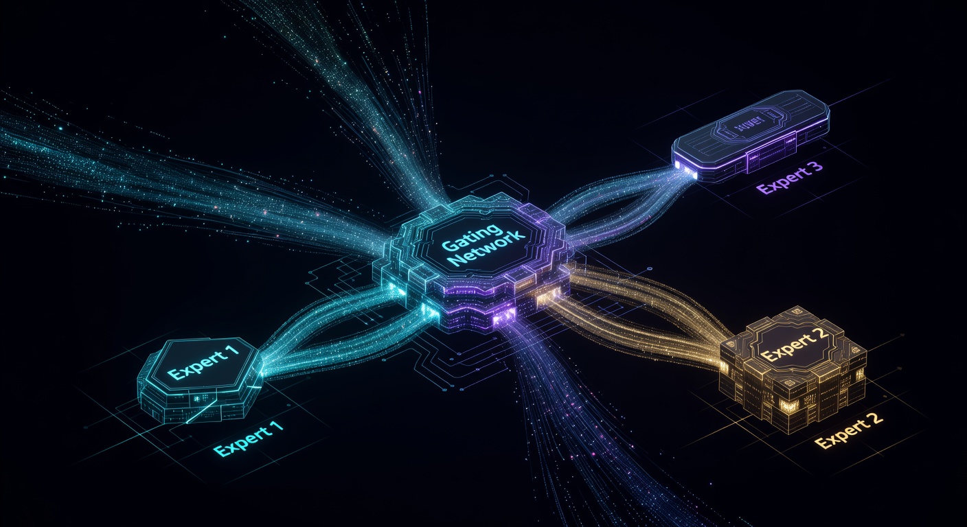
Imagine a Michelin-star kitchen where the recipe book has grown so large and specialized that no single chef — no matter how talented — can possibly master every technique at the level required. The solution the restaurant adopts is to hire a team of world-class specialists: a dedicated pastry chef, a grill master, a saucier, a sushi specialist, a fermentation expert, and so on. For any given dish, only two or three of these specialists actually touch the plate. The head chef (the "gating network") decides, based on the order coming in, which experts are needed for each component.

This is exactly the architecture behind modern Mixture-of-Experts (MoE) models — and it completely changes how you must think about model parallelism and serving infrastructure.

The Efficiency Promise of MoE

In a traditional dense model, every parameter is used for every token. In an MoE model, the total number of parameters can be enormous (hundreds of billions or even trillions), but only a small subset are activated for any given token.

Classic examples:

• Mixtral 8x7B: ~47B total parameters, but only ~12–13B active per token (2 experts out of 8).
• Grok-1 (314B): 8 experts, 2 active.
• DeepSeek-V2 / V3 and many frontier models: even more aggressive sparsity.

The result during training is dramatically better performance per FLOP. You get the capacity of a much larger model while only paying the compute cost of a smaller one. This is why so many of the strongest open-weight models in 2024–2025 are MoE architectures.

The Inference Reality: Token-Level Dynamic Routing

What makes MoE models beautiful for training makes them painful for inference if your infrastructure isn't designed for them.

In a dense model, the computation graph is static. Every token goes through exactly the same layers on the same GPUs.

In an MoE model:

• The attention layers are usually dense and replicated across all GPUs (everyone needs them).
• The feed-forward layers are replaced by many expert feed-forward networks.
• A small gating/router network looks at each token and decides which 1–2 (or top-k) experts should process it.
• Those tokens are then dispatched to the specific GPUs that hold the chosen experts.
• After the expert computation, the results are combined and sent back.

This dispatch-and-combine step happens at the granularity of individual tokens, inside the forward pass. It creates highly dynamic, data-dependent all-to-all communication patterns between GPUs that change on every single forward pass depending on the content of the prompt.

How Teams Actually Shard These Models

Common production strategies include:

• Replicate attention, shard experts: Attention layers live on every GPU. The expert weights are partitioned across the cluster. This is currently the most common approach.
• Expert parallelism + tensor parallelism combinations: Different dimensions of the problem are parallelized differently.
• Load balancing the experts: Because the gating network is content-dependent, some experts can become "hot" while others are idle. Good systems include auxiliary losses during training and runtime load-balancing techniques during inference.

The communication volume is significantly higher than in dense models. A naive implementation will spend more time moving tokens between GPUs than actually computing on them.

Why Generic Infrastructure Fails Here

Most traditional model servers assume a static computation graph. They have no concept of "this token needs to go to GPU 7 right now because that's where Expert 3 lives, while the next token from the same sequence needs to go to GPU 2."

This is why serving large MoE models on generic infrastructure is usually a painful, low-utilization experience. You need deep integration between the model architecture and the serving engine.

Today, the best support exists in:

• TensorRT-LLM (very strong MoE support from NVIDIA)
• vLLM and SGLang (rapidly improving, with good expert parallelism and dynamic routing)
• Custom internal stacks at the largest labs

Production Implications

If you are planning to serve (or fine-tune and then serve) one of the new generation of large open MoE models, you should assume from day one that you will need one of the specialized engines above. Trying to force it into a generic vLLM or Hugging Face Text Generation Inference setup without MoE-aware scheduling will leave large amounts of performance on the table and create operational headaches around load imbalance and communication overhead.

This is the final reason why "just use the same serving stack we used for our 7B model" almost never works at the frontier.

We have now walked through all five fundamental differences. Each one, by itself, is enough to make traditional serving infrastructure inefficient. Taken together, they explain why the industry has seen an explosion of specialized LLM inference engines and sophisticated orchestration layers. Let's bring it all together.

This is the practical takeaway of everything we've covered. Use it to audit your current inference stack, to evaluate a vendor or framework, or to pressure-test a proposed architecture before you bet your product on it.

Each item maps directly to one of the five fundamental differences. Check the box only if you can confidently say "yes, and here's how we do it well."

How to read your score:

• 5/5 — You are operating at a high level. You understand the five hard problems and have built (or chosen) systems that address them.
• 3–4/5 — A solid foundation. You have most of the basics in place; the remaining items are usually where the next round of cost or latency wins are hiding.
• 0–2/5 — You are still treating LLM serving like traditional model serving. Expect high costs, unpredictable latency, and scaling pain as traffic and context lengths grow.

If you have followed the story through all five sections, you should now see the kitchen with very different eyes.

You understand why the old fast-food model of serving (static batches, simple replication, round-robin routing, contiguous memory allocation) breaks down the moment you move beyond short, uniform, predictable requests.

You have seen how each of the five differences forces a fundamental change in how we think about compute, memory, and routing:

• Continuous batching turns the batch from a rigid group into a fluid, constantly reshuffling pool of work.
• Prefill–decode disaggregation acknowledges that preparing the ingredients and plating the dish have incompatible resource profiles and should often run on separate hardware.
• PagedAttention and modern KV cache management import decades of operating systems wisdom to solve the memory fragmentation problem that otherwise cripples long-context and high-concurrency serving.
• Prefix-aware routing treats the KV cache not as an implementation detail but as one of the most valuable assets in the entire system — one that must influence scheduling decisions.
• MoE-aware sharding and token-level routing forces us to abandon the idea of the model as a single static artifact and instead treat it as a dynamic, query-dependent distributed system.

Taken together, these changes represent a genuine phase shift in what it means to serve AI models at scale. The gap between "I can run this model on my laptop" and "I can serve this model to thousands of users with predictable latency and reasonable cost" is almost entirely explained by how deeply an engineering team understands and respects these five realities.

This is why we have seen an explosion of specialized inference engines (vLLM, SGLang, TensorRT-LLM, and others) and why orchestration layers like Ray have become so valuable — they provide the coordination fabric that lets these specialized components work together at scale.

As open-source models continue to push into the hundreds of billions and trillions of parameters, and as agentic and long-context applications become the norm rather than the exception, these distinctions will only become more important. Efficient inference is no longer just a cost optimization problem. In many cases it is a feasibility problem.

The teams that treat LLM serving as "just another model deployment" will continue to be surprised by their costs, their latency tails, and their inability to scale. The teams that internalize these five differences — and build (or choose) systems that are designed from the ground up around them — will be the ones who can actually deliver magical experiences at production scale without lighting money on fire.

You now have the mental model. The rest is execution.

This written piece expands significantly on a conversation I had while riding bikes (yes, really). The video version covers the high-level intuition. The post you're reading goes much deeper into mechanisms, numbers, and production implications.

• Kwon et al., "Efficient Memory Management for Large Language Model Serving with PagedAttention" (vLLM), SOSP 2023
• Yu et al., "Orca: A Distributed Serving System for Transformer-Based Generative Models," OSDI 2022
• SGLang papers and documentation (especially radix-tree prefix caching and disaggregation)
• TensorRT-LLM and Ray LLM documentation
• The Medium article on prefill vs decode stages (linked in original research)